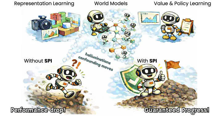
This blog post is based on our ICLR 2026 paper, Deep SPI: Safe Policy Improvement via World Models. You can also find the PDF, the code, and the poster.

In this post, I want to explain a simple tension in deep reinforcement learning: we often use auxiliary objectives to learn useful representations, but as soon as the policy changes, it becomes unclear whether the guarantees attached to the previous representation still say anything about the next one.

Deep SPI is our attempt to make that connection explicit. The core idea is to learn a world model together with a constrained policy-update rule, so that improving the policy in the model still guarantees improvement in the real environment up to a controlled error term, while the latent representation remains useful for the next policy as well.

Background

Deep RL starts from the familiar interaction loop: the agent acts, the environment transitions, and a reward comes back.

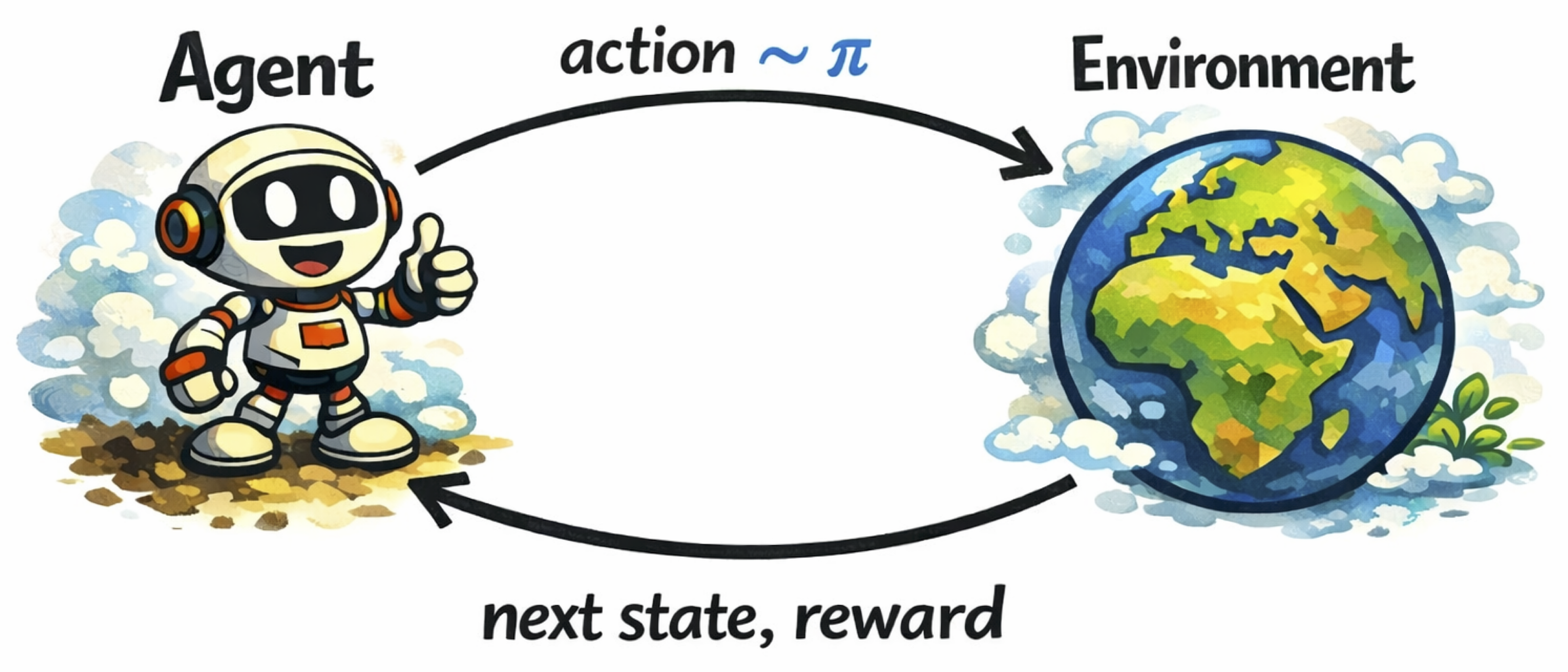
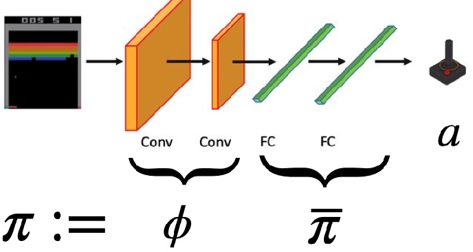
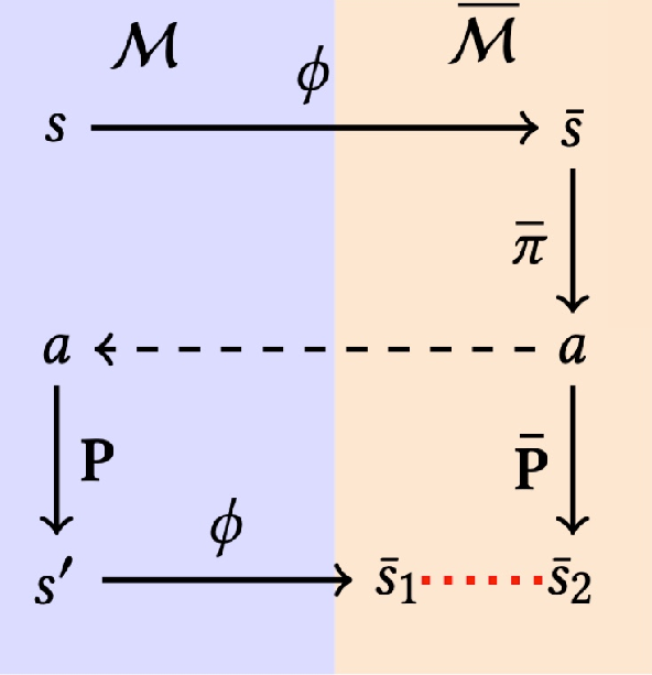
In modern settings, however, the agent does not act directly on a small symbolic state space. It acts on high-dimensional observations, such as Atari frames, so we first learn an encoder that maps the original state space $S$ to a latent space $\bar{S}$: $$ \phi \colon S \to \bar{S}. $$ The latent policy then acts on encoded states, $$ \bar{\pi} \colon \bar{S} \to \Delta(A), $$ and the deployed policy is the composition $$ \pi^{new} := \bar{\pi} \circ \phi. $$

What is a “good representation?”

For us, a good representation is not one that merely reconstructs images well. It is a representation that preserves what matters for control, namely the value induced by the policy we will actually deploy.

That is why the right quantity to keep in mind is $$ V^{\pi^{new}}(s) := \mathbb{E}\left[\sum_{t = 0}^{\infty} \gamma^t R(s_t, {\color{red}a_t}) \mid s_0 = s, \quad {\color{red}a_t} \sim \bar{\pi}(\phi(s_t))\right]. $$ If two states are close in latent space, their values should also remain close, at least up to a controlled error. This is the property that makes value approximation, planning, and generalization meaningful.

The catch is that most auxiliary guarantees are derived on-policy. So even if the current encoder is good for the current policy, updating both can immediately invalidate the old guarantee. That is the real problem Deep SPI is built to solve.

No Way Home: When World Models and Policies Go Out of Trajectories

World models are a natural place to attack the problem because they give us two useful objects at once: a reward predictor and a transition predictor. That makes them attractive both as auxiliary tasks for learning a representation and as models in which we can plan.

But there is an obvious danger. If the world model is trained on trajectories collected under a baseline policy $\pi_b$, then it can look good exactly where $\pi_b$ goes and still be badly wrong where the next policy wants to go.

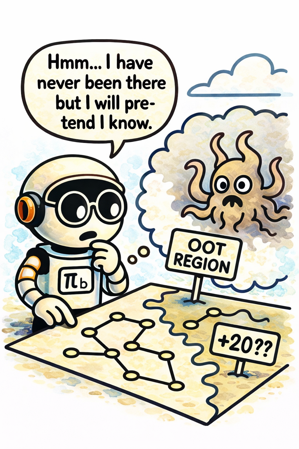
This is the out-of-trajectory problem. The issue is not that the model is globally useless; it is that it may be miscalibrated exactly in the region that suddenly matters for the new policy. Once that happens, planning inside the model can become optimistic for the wrong reasons.

So the question becomes: how do we keep policy updates close enough to the data regime that shaped the world model, while still making progress?

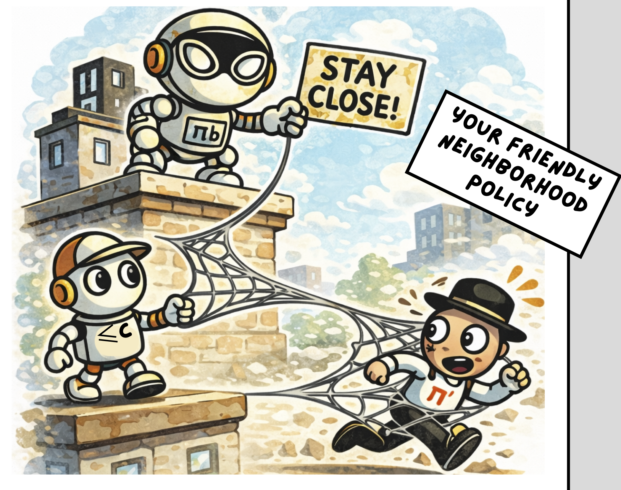
Your Friendly Neighborhood Policy

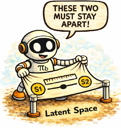
The answer in the paper is to introduce a neighborhood operator around the current policy. Instead of allowing an arbitrary jump from $\pi_b$ to a new policy $\pi$, we only consider policies whose action probabilities remain inside a trust region defined by importance-ratio bounds.

Formally, $$ \mathcal{N}^{C}(\pi_b) := \left{ \pi ;:; 2 - C \le \frac{\pi(a \mid s)}{\pi_b(a \mid s)} \le C \text{ for all } s \text{ and all } a \in \mathrm{supp}(\pi_b(\cdot \mid s)) \right}. $$ So $\mathcal{N}^{C}(\pi_b)$ is the neighborhood of policies whose action probabilities remain in the ratio band $[2 - C, C]$ relative to the baseline policy. The update rule then becomes $$ \pi_{n+1} \in \arg\max_{\pi \in \mathcal{N}^{C}(\pi_n)} \mathbb{E}_{s \sim d^{\pi_n},, a \sim \pi(\cdot \mid s)}\left[A^{\pi_n}(s, a)\right]. $$

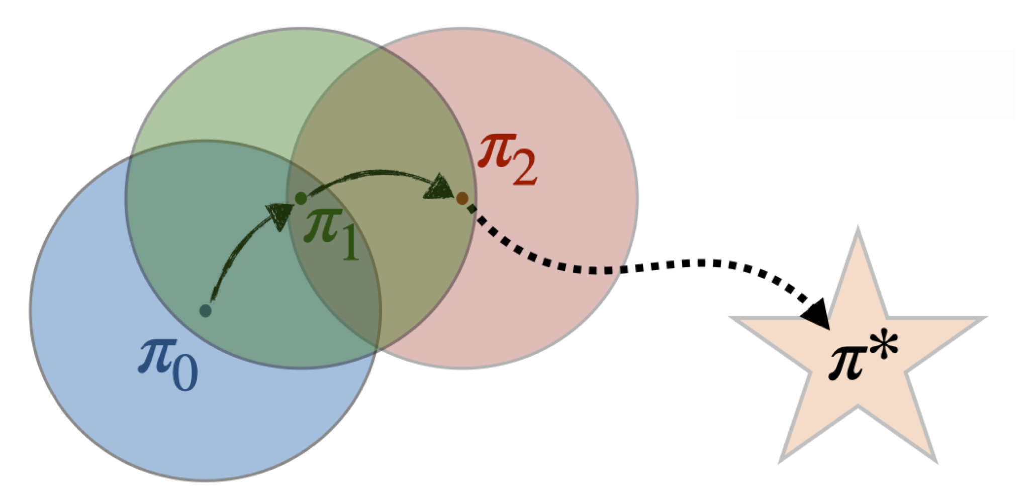
Why is this useful? Because once updates are local, Deep SPI inherits the key safe-policy-improvement story: iterative updates improve monotonically, the sequence converges, and the next policy cannot drift arbitrarily far from the data regime that made the current world model and representation meaningful.

This is also why I like the mirror-descent picture so much. Deep SPI is not about one giant policy leap. It is about a sequence of small, trustworthy moves.

With Great World Models Comes Great Representation

Once updates are local, we can ask a more refined question: what should the world model actually learn?

Learning a sound world model

Deep SPI uses a reward loss and a transition loss tied to the baseline policy’s data. For the reward we use an $L_1$ prediction loss, and for the transition dynamics we may simply use a Euclidean norm in latent space (this is already sufficient for the guarantee, though tighter bounds may come from a more elaborate Wasserstein loss as in WAE-MDPs):

$$ L_R := \mathbb{E}{(s,a,r_t)\sim \pi_b}\left[\left|r_t - \bar R(\phi(s), a)\right|\right] $$ $$ \color{red}{L_P := \mathbb{E}{(s,a,s’)\sim \pi_b}\left[\mathbb{E}_{s^+ \sim \bar P(\cdot \mid \phi(s), a)}\left[\lVert \phi(s’) - s^+ \rVert_2\right]\right]} $$

The important point is that these are local losses. They are measured on the state-action distribution induced by the baseline policy, so they are exactly the quantities that tell us whether the world model is calibrated in the region where we currently have data.

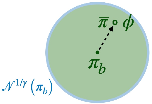
Restricting the policy update for the next two guarantees

From this point on, the next two guarantees use the stricter neighborhood $$ \pi^{new} \in \mathcal{N}^{1/\gamma}(\pi_b). $$ This is where the discount factor becomes more than just an RL convenience: it defines an implicit horizon, or if you prefer an implicit radius, for the policy update scheme. Smaller effective horizons permit larger safe deviations, while larger horizons force the update to stay tighter. The next theorems are important precisely because they hold under this particular constraint.

Deep safe policy improvement

Under that controlled update regime, the paper proves the key transfer statement: if the policy improves enough in the world model, then it also improves in the real environment up to a local model-error term.

Define the real-environment value and the latent-model value as $$ V^{\pi}(s) := \mathbb{E}{\mathcal{M},\pi}\left[\sum{t=0}^{\infty}\gamma^t r_t \mid s_0 = s\right], \qquad \bar{V}^{\bar{\pi}}(\bar{s}) := \mathbb{E}{\bar{\mathcal{M}},\bar{\pi}}\left[\sum{t=0}^{\infty}\gamma^t \bar{r}_t \mid \bar{s}_0 = \bar{s}\right]. $$ Then the Deep SPI guarantee can be read as $$ V^{\pi^{new}}(s) - V^{\pi_b}(s) \ge \bar{V}^{\bar{\pi}}(\phi(s)) - \bar{V}^{\bar{\pi}_b}(\phi(s)) - \zeta_b, $$ where $\pi^{new} = \bar{\pi} \circ \phi$ and $\zeta_b$ is the local model error induced by the losses $L_R^{\pi_b}$ and $L_P^{\pi_b}$.

That is the central SPI message of the paper: model-based improvement is not just a heuristic anymore. As long as the world model is accurate enough on the baseline-policy data and the update stays inside the safe neighborhood, any gain in the world model transfers back to the real environment.

Deep SPI for representation learning

The representation-learning theorem is the part I find especially satisfying. It says that under the same controlled policy change, the learned latent space remains almost Lipschitz for the next policy: $$ \left|V^{\pi}(s_1) - V^{\pi}(s_2)\right| \le K_V , \left|\phi(s_1) - \phi(s_2)\right|_2 + \varepsilon, \qquad \text{for all } \pi \in \mathcal{N}^{1/\gamma}(\pi_b), $$ with probability at least $1-\delta_b$, where $\delta_b$ is controlled by the local losses $L_R^{\pi_b}$ and $L_P^{\pi_b}$.

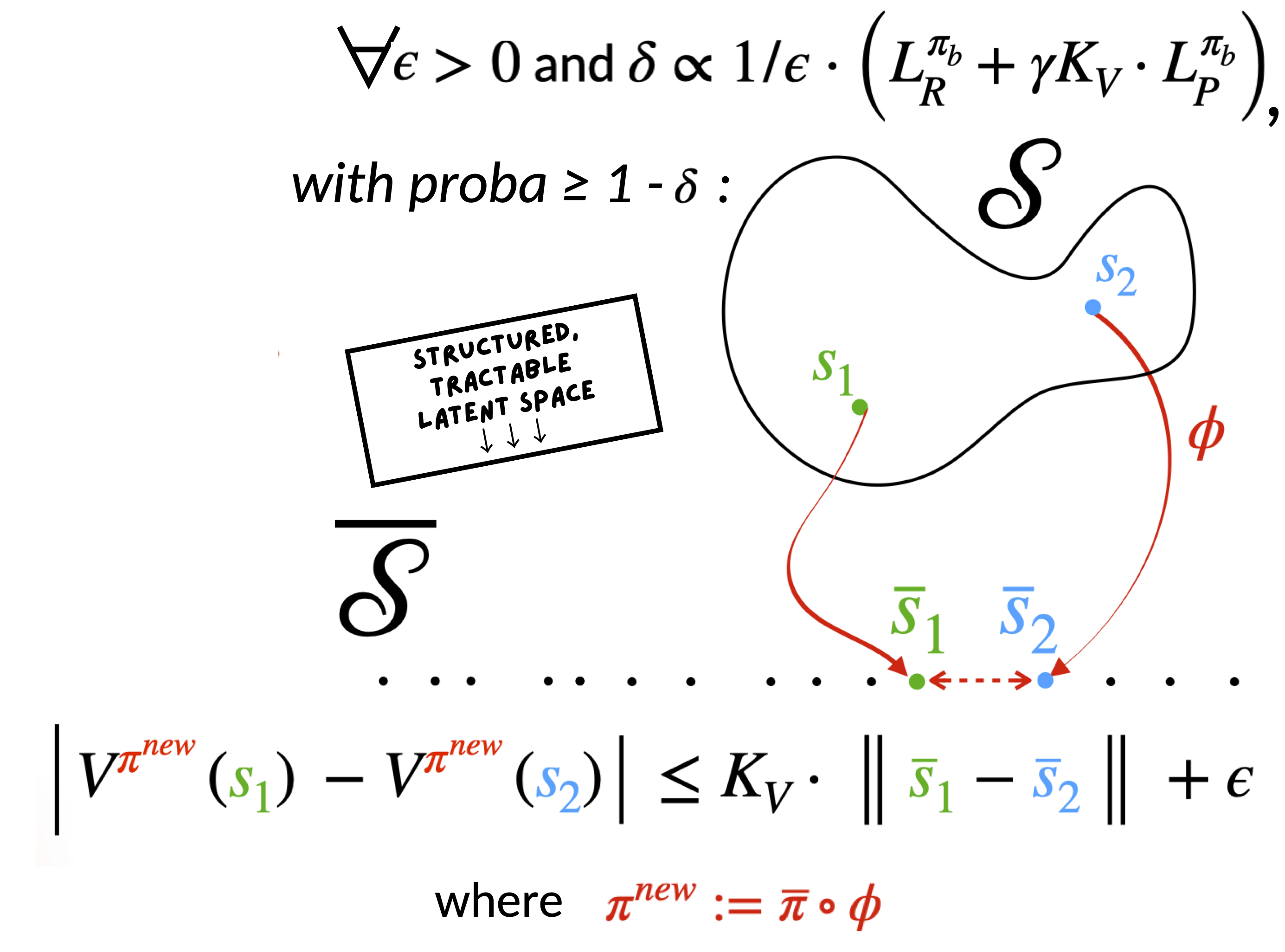
Why is that good? Because it says the latent geometry is still informative for value after the policy update. That helps value approximation and planning, but it also says something important about representation collapse: if two states have very different values, the theorem prevents the encoder from mapping them all to the same latent point while keeping the guarantee intact. So the result is useful both positively, for generalization, and negatively, because it rules out a degenerate failure mode.

Across the SPI-Verse: PPO Comes Into Play

The theory naturally raises a practical question: how do we enforce the neighborhood in a modern deep RL pipeline?

PPO is the natural answer. Its clipped objective already behaves like a trust-region heuristic, so Deep SPI starts from PPO and modifies it in a way that keeps the neighborhood logic intact.

The naive idea would be to add the world-model losses directly to the PPO loss. But that would be wrong. Those losses update the encoder, so they can indirectly push the composed policy $\bar{\pi} \circ \phi$ outside the neighborhood even if the policy head alone still looks well behaved.

The fix is to fold the auxiliary terms into the utility itself: $$ U^{\pi_n}(s_t, a_t, s_{t+1}) := A^{\pi_n}(s_t, a_t) - \alpha_R L_R - \alpha_P L_P $$ and then optimize the PPO-like objective $$ L_{\mathrm{DeepSPI}}(\pi) := \mathbb{E}\left[ \min\left( r_t(\pi) U_t,, \operatorname{clip}(r_t(\pi), 1-\varepsilon, 1+\varepsilon) U_t \right) \right], $$ where $$ r_t(\pi) := \frac{\pi(a_t \mid s_t)}{\pi_n(a_t \mid s_t)}. $$ In this PPO-like relaxation, we choose the clipping parameter to match the neighborhood scale, namely $$ \varepsilon = C - 1. $$ So Deep SPI keeps PPO’s trust-region behavior while making the world-model terms part of the very quantity whose local improvement is being optimized.

There is also a very practical data issue here. PPO is on-policy, which means world-model learning can easily suffer from narrow, highly correlated coverage if we collect long rollouts from only a few environments. That is exactly the wrong regime for learning a calibrated world model.

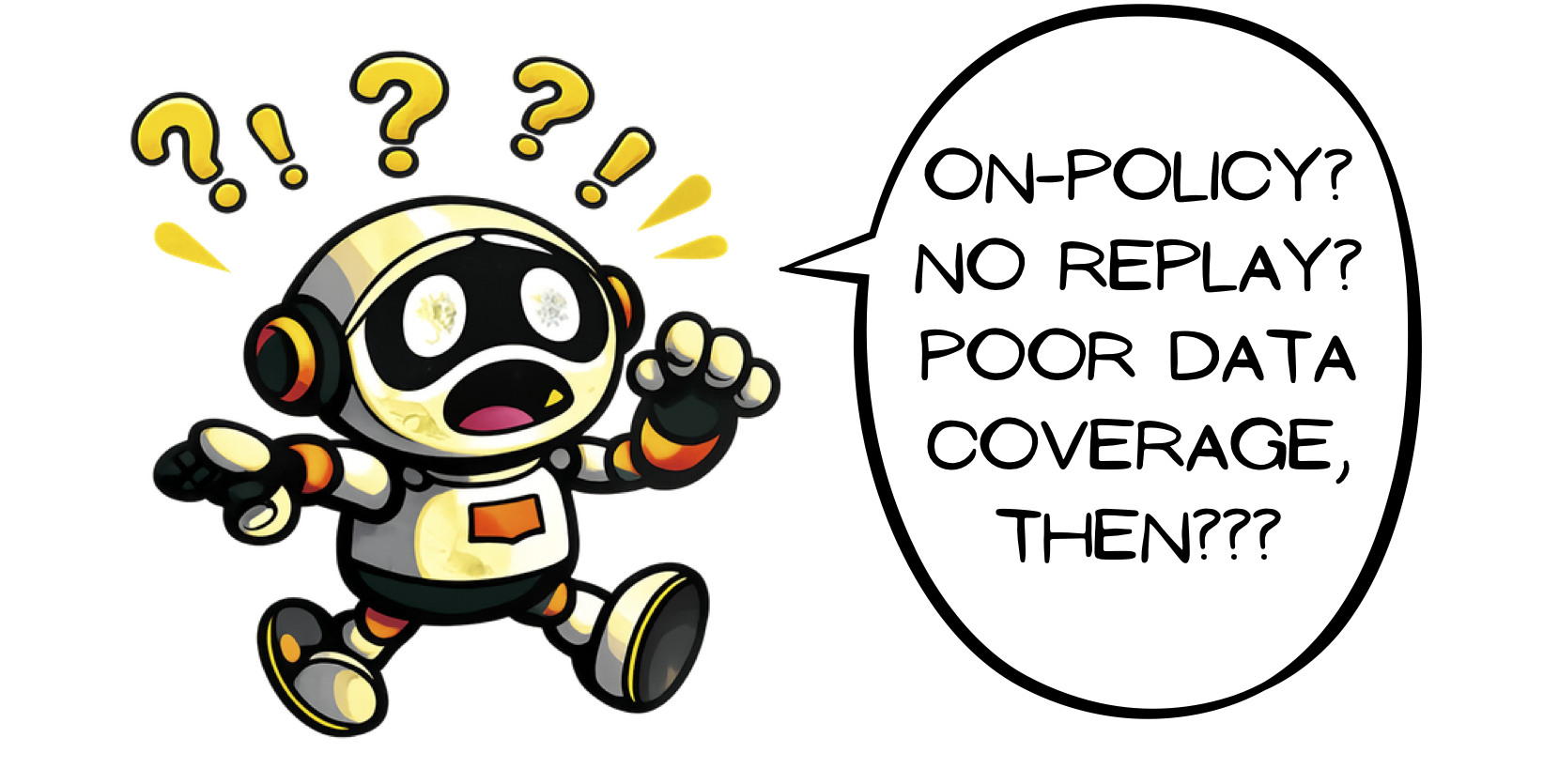
In practice, the JAX implementation matters a lot here. The move from a handful of environments with long rollouts to many environments with short rollouts gives much broader state coverage without abandoning the on-policy setup. That detail is easy to miss when reading only the theorem statements, but it is critical in the actual algorithm: a local guarantee is only helpful if the local data cover enough of the neighborhood to learn the model well.

Experiments

The payoff is that Deep SPI is not only theoretically neat. On 57 stochastic Atari environments, it is also competitive with strong baselines such as PPO and DeepMDPs.

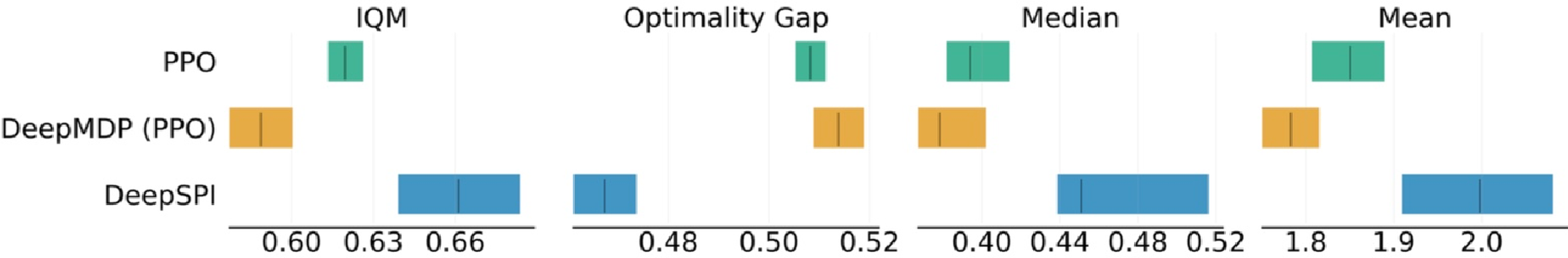
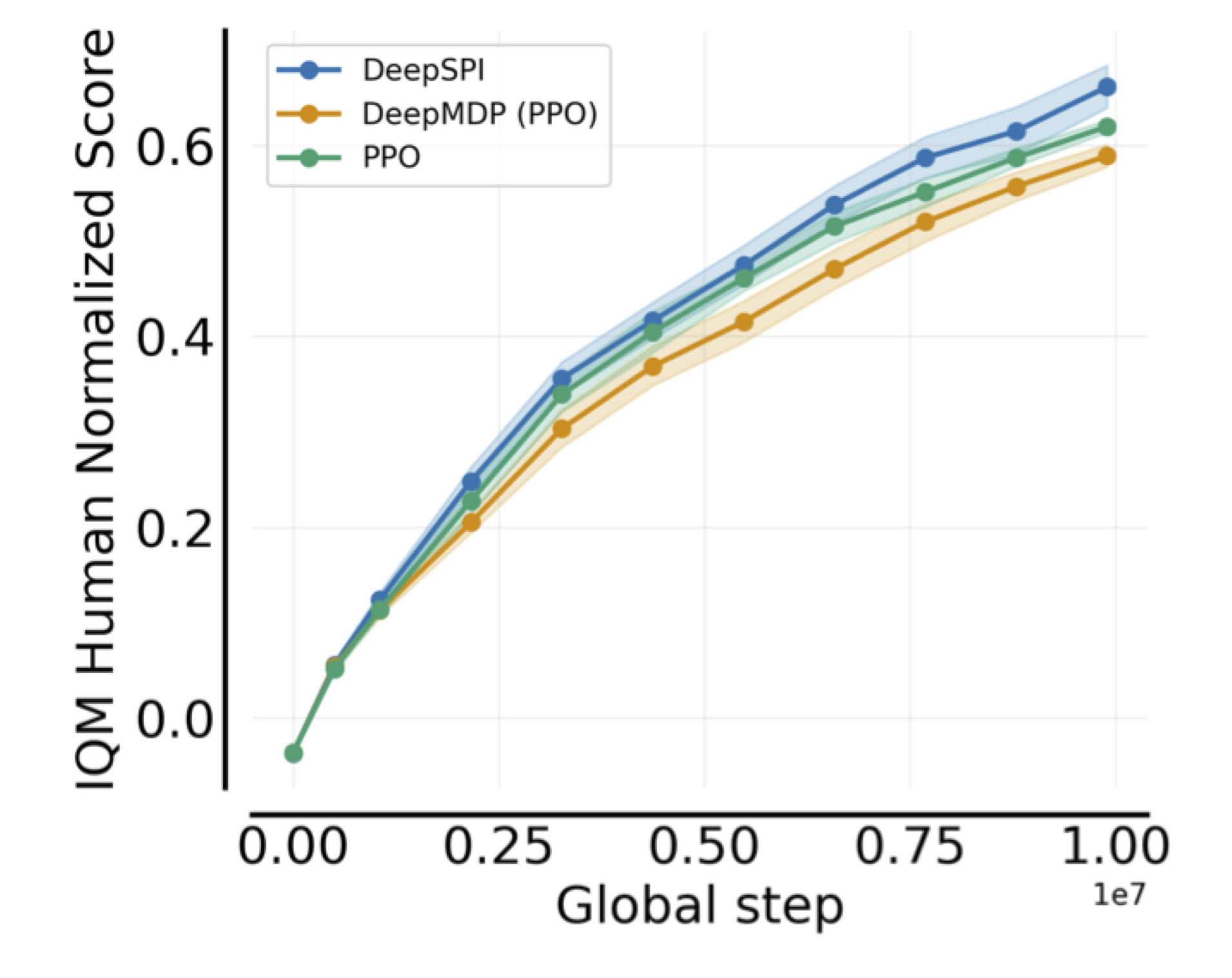
What I like about these results is that they line up with the theory. The method is not competitive in spite of the neighborhood/world-model discipline. It is competitive because that discipline prevents the update from breaking the very representation and model assumptions the algorithm relies on.

Conclusion and Future Work

The central claim of Deep SPI is that policy improvement, world-model calibration, and representation learning should not be treated as separate problems. If the representation is supposed to support policy improvement, then the update rule itself has to appear in the analysis.

That is why the neighborhood constraint matters so much. It is the bridge that lets us say, in a deep RL setting, that model-based improvement is reliable up to controlled local error, and that the representation learned today can still be useful for the next policy tomorrow.

More broadly, I think this is a useful perspective on world models in RL. They are not only tools for sample efficiency; they can also be tools for reliable policy improvement. That is the perspective behind Deep SPI, and I expect it will matter even more as world-model-based agents become larger, more general, and more autonomous.