Implementation of the techniques presented in our paper Deep SPI: Safe Policy Improvement via World Models.
- Code: GitHub repository
- Paper: ICLR 2026
- Blog: Deep SPI explainer
The Core Problem
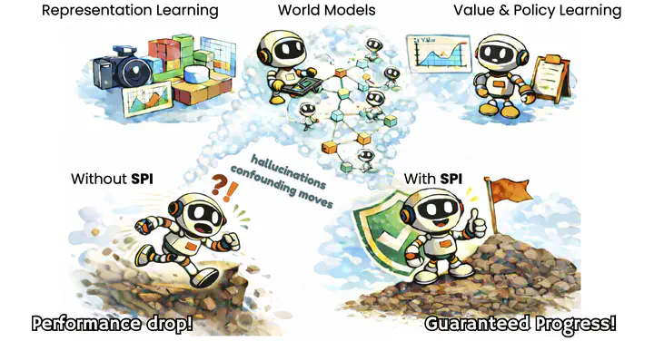
When you train a deep RL policy with auxiliary losses to improve the representation (the observation encoder before your value/critic heads), you face a critical timing problem: The representation optimized under your behavioral policy may not be reliable for the next policy. Add auxiliary losses to regularize the latent space, improve the policy, and suddenly the encoder has shifted, invalidating the very representation you were relying on.
Deep SPI solves this by coupling world-model learning with controlled policy updates: you improve the policy step by step, in a neighborhood that keeps it close to regions where the world model is well-calibrated. This way, updates that look good in the model actually translate to improvements in the real environment.
How It Works: The Algorithm
Deep SPI operates on a deep RL agent where the learned representation $\phi$ (the encoder) maps raw observations into a compact latent space. This representation is shared by both the policy and the world model—the policy predicts actions from $\phi(s)$, and the world model predicts rewards and transitions from $\phi(s)$. The core insight is that as the policy improves, this shared representation can shift, breaking the world model’s calibration. Deep SPI solves this by constraining policy updates to stay in a neighborhood where the world model remains reliable.
Learning a Reliable World Model
Learn two predictors $\overline{R}$ (reward) and $\overline{P}$ (transition) on behavioral data, operating on the learned representation $\phi(s)$:
These measure calibration exactly where you have data, telling you whether the model is reliable for the next policy update.
Enforcing a Policy Neighborhood
Restrict new policies to stay close to the current policy: action probabilities can’t deviate more than a fixed ratio (similar to PPO’s clipping). This keeps updates close to the data regime, ensuring the world model remains trustworthy.
The Core Guarantee
With constrained updates and small prediction losses, improvements in the learned model transfer back to the real environment. The gap between model and reality shrinks as the prediction losses shrink — so if you’re predicting rewards and transitions well, your planned improvements will actually happen in the real world.
Representation Quality
The encoder remains useful for the next policy: states with very different values can’t collapse to the same latent point without breaking the guarantee. This prevents representation degradation and keeps the learned state abstraction useful as you improve the policy.
Implementation: PPO + World Models
The practical question: how do you enforce the neighborhood in a modern deep RL pipeline?
The answer is PPO, because its clipped objective already acts like a trust region. We build upon Clean RL implementations for robust JAX-based training. But there’s a critical subtlety: auxiliary losses (like $L_R$ and $L_P$) update the encoder, so they can indirectly push the composed policy $\pi := \bar{\pi} \circ \phi$ outside the neighborhood even if the policy head looks well-behaved.
The fix: fold the auxiliary terms into the advantage function $A(s, a)$:
$$ U(s, a) := A(s, a) - \alpha_R \cdot L_R - \alpha_P \cdot L_P $$
Then optimize a PPO-like objective. This way, the encoder and policy head move together in a way that respects the neighborhood constraint.
The Data Coverage Problem
There’s a critical practical detail: PPO is on-policy, which means world-model learning can suffer from narrow, correlated coverage if you collect long rollouts from only a few environments. That’s exactly the wrong regime for learning a well-calibrated world model.
The solution: use many vectorized JAX environments with shorter rollouts instead of a few environments with long rollouts. This gives much broader state coverage while staying on-policy—crucial because a local guarantee is only helpful if your local data actually cover enough of the neighborhood to learn the model well.
Implementation Details
- Framework: JAX-based, for efficient jitted computation and GPU scaling
- Vectorized environments: many parallel JAX-jitted environments with shorter rollouts for better state coverage
- Reproducibility: checked-in
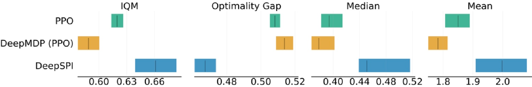
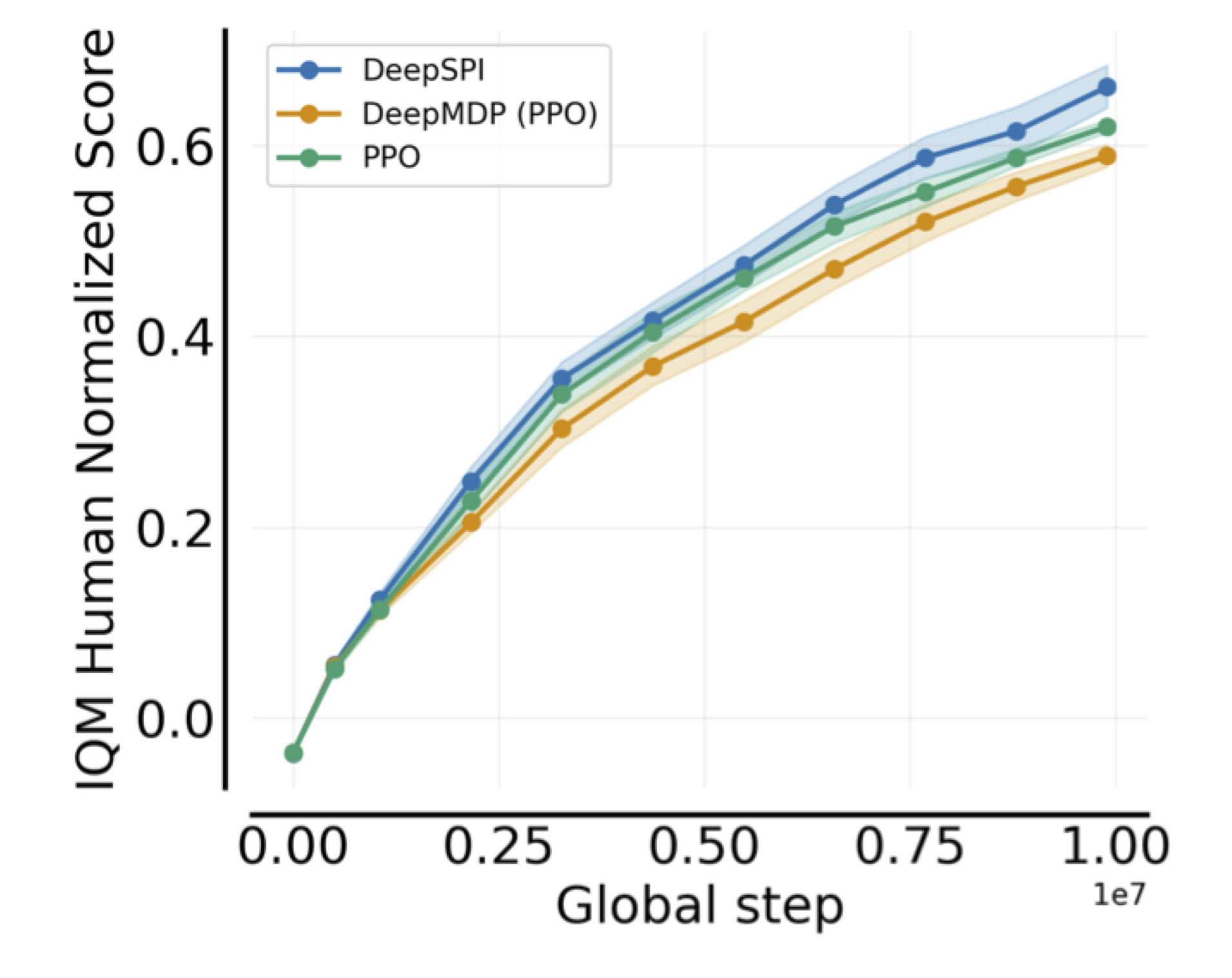
uv.lockfor exact dependency reproducibility - Benchmarks: ALE-57 (57 Atari games), with results matching or exceeding PPO and DeepMDPs
- Environments: uses
envpoolfor high-throughput Atari simulation with GPU support - Code structure: modular design separating encoder, policy, world model, and PPO training logic
Why It Matters
Most auxiliary-loss approaches (even VAE-MDPs and related work) derive their guarantees on-policy, meaning they are valid only for the policy that collected the data. Deep SPI extends this to show that with controlled updates, the guarantees survive the policy change. This is especially valuable because:
- Monotonic improvement: You can reason about whether each update actually helps, not just whether it looks good in hindsight
- Representation stability: The encoder doesn’t degrade as you improve the policy—it stays useful for downstream learning
- No offline requirement: Deep SPI works in online settings; you don’t need a pre-collected dataset
Results
On ALE-57, Deep SPI matches or exceeds PPO and DeepMDPs while maintaining explicit monotonic improvement bounds. The algorithm demonstrates that principled methods with guarantees and practical performance need not be in tension.
Learn More
- Paper: Deep SPI: Safe Policy Improvement via World Models (ICLR 2026)
- Blog post: Deep SPI explainer with visualizations and detailed worked examples
- Code: GitHub repository with reproducible setup and Atari experiments